QAOA Ansatz – Max-κ-ColorableSubgraph

This ansatz follows the feasible-subspace QAOA construction of Section 4.1 in Hadfield et al., arXiv:1709.03489.

Each graph node is encoded using a one-hot register of (κ) qubits, and the mixer Hamiltonian is chosen to preserve Hamming weight, ensuring that the quantum state remains within the valid coloring subspace throughout the evolution.

from functools import partial, reduce
from operator import add
from time import perf_counter
from ket import *
from scipy.optimize import minimize as scipy_minimize
import networkx as nx
import matplotlib.pyplot as plt

SIMULATOR = "sparse"

def mixer_h(nodes: list[Quant]) -> Hamiltonian:
    """
    Constructs the Mixer Hamiltonian (H_M) using an XY-Mixer.

    In the context of the one-hot encoding used here (where each node has k qubits
    but only one is allowed to be |1>), the XY mixer preserves the Hamming weight.
    This ensures that the quantum state remains within the valid subspace (valid colorings)
    throughout the evolution, provided the initial state is valid.

    Args:
        nodes: A list of quantum registers (Quant), where each register
               represents a graph node.

    Returns:
        The Hamiltonian observable for the mixer.
    """
    k = len(nodes[0])

    with obs():
        return sum(
            sum(
                X(node[i]) * X(node[(i + 1) % k]) + Y(node[i]) * Y(node[(i + 1) % k])
                for i in range(k)
            )
            / 2
            for node in nodes
        )

def cost_h(nodes: list[Quant], graph: list[(int, int)]) -> Hamiltonian:
    """
    Constructs the Cost Hamiltonian (H_C) for the Graph Coloring problem.

    The Hamiltonian adds an energy penalty if two connected nodes (u, v) have
    the same active color index.

    Args:
        nodes: A list of quantum registers allocated for the graph nodes.
        graph: A list of tuples (u, v) representing graph edges.

    Returns:
        The Hamiltonian observable for the cost function.
    """
    k = len(nodes[0])  # Number of colors (qubits per node)
    with obs():
        # Correlates Z operators on connected nodes at the same color index.
        # If qubits are identical (both 0 or both 1), it contributes to energy.
        # Since valid states are 1-hot, this effectively penalizes same-color collisions.
        return len(graph) - (
            sum(
                sum((1 - Z(nodes[u][a]) * Z(nodes[v][a])) for a in range(k))
                for (u, v) in graph
            )
            / 4
        )

def cost(graph: list[(int, int)], n: int, k: int, colors: list[int]) -> float:
    """
    Calculates the energy cost for a specific classical color assignment.

    This is used during post-processing to verify the cost of the results found
    by the quantum algorithm.

    Args:
        graph: The edge list of the graph.
        n: Number of nodes.
        k: Number of colors.
        colors: A list of integers, where each integer acts as a bitmask
                representing the one-hot state of a node (e.g., 4 -> '100').

    Returns:
        The expectation value (energy) of the configuration.
    """
    p = Process(execution="batch", simulator=SIMULATOR, num_qubits=n * k)
    nodes = [p.alloc(k) for _ in range(n)]

    # Initialize the specific classical state based on the input colors
    for node, color in zip(nodes, colors):
        # f"{color:0{k}b}" converts int color to binary string of length k
        for qubit, bit in zip(node, f"{color:0{k}b}"):
            if bit == "1":
                X(qubit)
                continue

    return exp_value(cost_h(nodes, graph)).get()

def initial_state(nodes: list[Quant]):
    """
    Prepares the initial quantum state |psi_0>.

    Sets the 0-th qubit of every node to |1> and the rest to |0>.
    State: |100...0>_1 |100...0>_2 ...
    This is a valid One-Hot encoding (Color 0 is initially selected for all nodes).

    Args:
        nodes: The list of quantum registers.
    """
    for node in nodes:
        X(node[0])

def QAOA_ansatz(
    nodes: list[Quant], graph: list[(int, int)], gamma: list[float], beta: list[float]
):
    """
    Applies the QAOA variational circuit layers.

    Args:
        nodes: The quantum registers.
        graph: The graph edge list.
        gamma: List of rotation angles for the Cost Hamiltonian.
        beta: List of rotation angles for the Mixer Hamiltonian.
    """
    initial_state(nodes)

    # Pre-evolution step (Specific strategy for this ansatz)
    evolve(beta[-1] * mixer_h(nodes))

    for g, b in zip(gamma, beta):
        evolve(g * cost_h(nodes, graph))
        evolve(b * mixer_h(nodes))

def call_QAOA_ansatz(
    graph: list[(int, int)], n: int, k: int, parameters: list[float]
) -> list[Quant]:
    """
    Allocates the process and constructs the QAOA circuit.

    Args:
        graph: The graph structure.
        n: Number of nodes.
        k: Number of colors.
        parameters: Concatenated list of [gamma..., beta...].

    Returns:
        The allocated quantum variables with the circuit applied.
    """
    # Split parameters into gamma and beta
    # Note: The logic assumes len(params) = 2*l + 1 based on slicing logic
    l = (len(parameters) - 1) // 2
    gamma = parameters[:l]
    beta = parameters[l:]

    p = Process(execution="batch", simulator=SIMULATOR, num_qubits=n * k)
    nodes = [p.alloc(k) for _ in range(n)]
    QAOA_ansatz(nodes, graph, gamma, beta)
    return nodes

def objective(
    graph: list[(int, int)], n: int, k: int, parameters: list[float]
) -> float:
    """
    The objective function to minimize. Calculates the expectation value of the
    Cost Hamiltonian given the current parameters.

    Args:
        graph: The graph edge list.
        n: Number of nodes.
        k: Number of colors.
        parameters: Optimization parameters.

    Returns:
        The expected energy (cost).
    """
    begin = perf_counter()
    nodes = call_QAOA_ansatz(graph, n, k, parameters)
    c = exp_value(cost_h(nodes, graph)).get()
    end = perf_counter()

    # Real-time logging of optimization progress overwriting the same line
    print(f"Current Cost: {c:+.6f} ({end-begin:.4f}s)", end="\r", flush=True)

    return c

def final_result(
    graph: list[(int, int)], n: int, k: int, parameters: list[float]
) -> Samples:
    """
    Runs the circuit with the optimal parameters found and samples the output.

    Args:
        graph: The graph edge list.
        n: Number of nodes.
        k: Number of colors.
        parameters: Optimal parameters found by minimization.

    Returns:
        An object containing measurement samples.
    """
    # 'reduce(add, ...)' concatenates all qubit registers into one large register
    # so we can sample the entire system state at once.
    nodes = reduce(add, call_QAOA_ansatz(graph, n, k, parameters))

    return sample(nodes, 100)


def from_one_hot_to_int(value: int) -> int | None:
    """
    Converts a One-Hot integer representation to a simple color index.

    Example:
        If k=4 and value is '0100' (binary 4), it returns 3 (length of '100').
        This maps the one-hot position to a color ID.

    Args:
        value: Integer resulting from measuring k qubits.

    Returns:
        The index of the color, or None if the state
        was not one-hot (invalid).
    """
    if value.bit_count() == 1:
        return value.bit_length()
    else:
        return None


def postprocessing(result: dict[int, int], graph: list[(int, int)], n: int, k: int):
    """
    Processes raw measurement counts into human-readable results.

    Args:
        result): Dictionary of {state_int: count}.
        graph: Graph structure.
        n: Number of nodes.
        k: Number of colors.

    Returns:
        A list of tuples containing:
        (Decoded Colors Tuple, Count, Cost/Energy, Raw One-Hot Tuples)
    """
    total_qubits = n * k

    # Break down the large integer measurement (representing n*k qubits)
    # into n separate integers (each representing k qubits for one node)
    one_hot_colors = [
        tuple(
            int(f"{state:0{total_qubits}b}"[i * k : (i + 1) * k], 2) for i in range(n)
        )
        for state in result.keys()
    ]

    # Convert one-hot ints to human-readable color indices
    int_colors = [
        tuple(from_one_hot_to_int(c) for c in color) for color in one_hot_colors
    ]

    # Calculate exact cost for each found configuration to verify quality
    cost_colors = [cost(graph, n, k, color) for color in one_hot_colors]

    return list(zip(int_colors, list(result.values()), cost_colors, one_hot_colors))


def plot_colored_graph(graph: list[(int, int)], colors: list[int]):
    """
    Visualizes the graph with nodes colored according to the result.

    Args:
        edges: The graph edges.
        color_indices: List of color IDs for the nodes.
    """
    G = nx.Graph()
    G.add_edges_from(graph)

    palette = {
        1: "#FFC1C1",
        2: "#C1E1C1",
        3: "#BEE7FF",
        4: "#FFD8A8",
        5: "#FFF2A8",
        6: "#D4C1FF",
        7: "#C1FFF0",
        8: "#E8C1FF",
        9: "#CCE5FF",
        10: "#F2E6C9",
    }

    final_colors = []
    for node in G.nodes():
        color_code = colors[node]
        final_colors.append(palette.get(color_code, "#737373"))

    plt.figure(figsize=(6, 6))
    pos = nx.spring_layout(G, seed=42)

    nx.draw(
        G,
        pos,
        with_labels=True,
        node_color=final_colors,
        node_size=2000,
        edge_color="gray",
        font_weight="bold",
        width=2,
    )

    plt.show()

def minimize(graph: list[(int, int)], n: int, k: int, l: int, maxiter: int = 300):
    """
    Main driver function to run the QAOA optimization loop.

    Args:
        graph: Graph edges.
        n: Number of nodes.
        k: Number of colors.
        l: Number of QAOA layers (p).
        maxiter: Maximum iterations for the classical optimizer.

    Returns:
        tuple: (Optimization Result, Processed Results List)
    """
    # Initialize parameters.
    # Size is (2*l + 1) because the ansatz uses a specific pre-evolution step
    # or the slicing logic in `call_QAOA_ansatz` expects it.
    parameters = [0.5 for _ in range(2 * l + 1)]

    res = scipy_minimize(
        partial(objective, graph, n, k),
        parameters,
        method="COBYLA",
        options={"maxiter": maxiter},
    )

    # Get final samples using the optimized parameters
    result = final_result(graph, n, k, res.x).get()

    # Process and sort results by cost (lowest energy first)
    result = sorted(postprocessing(result, graph, n, k), key=lambda a: a[2])

    return res, result

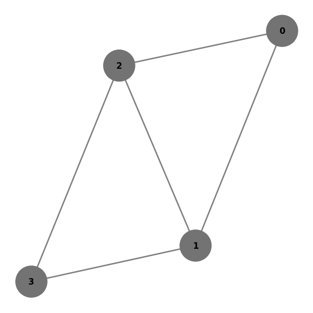
graph = [(0, 1), (0, 2), (1, 2), (1, 3), (2, 3)]
n = 4
m = len(graph)
k = 3
l = 4

plot_colored_graph(graph, [None for _ in range(n)])

res, result = minimize(graph, n, k, l)
print(res)

print_n_results = 2

print("Sorted by cost")
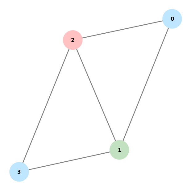
for i, color in enumerate(result[:print_n_results]):
    print(f"{i}: Count={color[1]} Cost={color[2]} Color={color[3]}")
    plot_colored_graph(graph, color[0])

 message: Return from COBYLA because the objective function has been evaluated MAXFUN times.
 success: False
  status: 3
     fun: 0.8732539417581898
       x: [ 1.297e+00  8.002e-01  1.447e+00  6.308e-01  1.364e+00
            1.107e+00  6.173e-01  1.390e+00  6.464e-01]
    nfev: 300
   maxcv: 0.0
Sorted by cost
0: Count=15 Cost=0.0 Color=(1, 4, 2, 1)

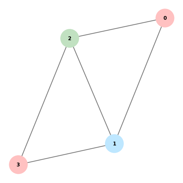
1: Count=5 Cost=0.0 Color=(4, 2, 1, 4)

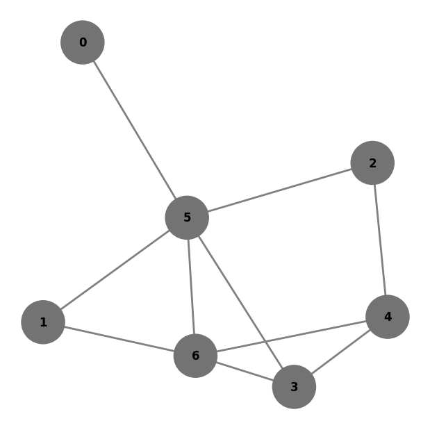
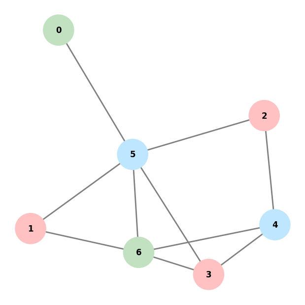
graph = [(0, 5), (1, 5), (1, 6), (2, 4), (2, 5), (3, 4), (3, 5), (3, 6), (4, 6), (5, 6)]
n = 7
k = 3
m = len(graph)
l = 4

plot_colored_graph(graph, [None for _ in range(n)])

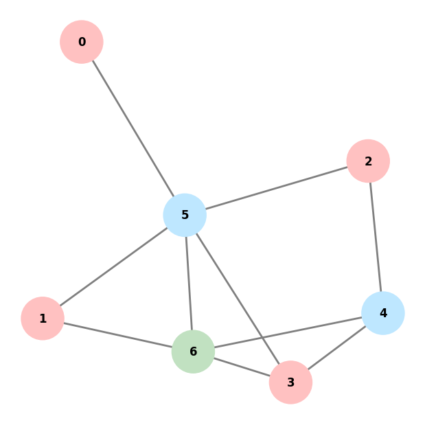
res, result = minimize(graph, n, k, l)
print(res)

print_n_results = 2

print("Sorted by cost")
for i, color in enumerate(result[:print_n_results]):
    print(f"{i}: Count={color[1]} Cost={color[2]} Color={color[3]}")
    plot_colored_graph(graph, color[0])

 message: Return from COBYLA because the objective function has been evaluated MAXFUN times.
 success: False
  status: 3
     fun: 2.644479806886681
       x: [ 1.673e+00  1.556e+00  2.039e+00  6.673e-01  1.526e+00
            2.380e-02  9.710e-01  2.574e-01  1.552e-01]
    nfev: 300
   maxcv: 0.0
Sorted by cost
0: Count=1 Cost=0.0 Color=(2, 1, 1, 1, 4, 4, 2)

1: Count=1 Cost=0.0 Color=(1, 1, 1, 1, 4, 4, 2)

from ket import ket_version

ket_version()

['Ket v0.9.2.2b1',
 'libket v0.6.0 [rustc 1.92.0 (ded5c06cf 2025-12-08) x86_64-unknown-linux-gnu]',
 'kbw v0.4.2 [rustc 1.92.0 (ded5c06cf 2025-12-08) x86_64-unknown-linux-gnu]']