from typing import Callable
from functools import partial

from scipy.optimize import minimize, OptimizeResult
from IPython.display import display

import plotly.io as pio
pio.renderers.default = "notebook_connected"

from ket import *
from ket import ket_version

ket_version()
['Ket v0.10.1',
 'libket v0.7.1 [rustc 1.97.0 (2d8144b78 2026-07-07) x86_64-unknown-linux-gnu]',
 'kbw v0.5.1 [rustc 1.97.0 (2d8144b78 2026-07-07) x86_64-unknown-linux-gnu]']
Quantum Approximate Optimization Algorithm (QAOA)
The Quantum Approximate Optimization Algorithm (QAOA) is a hybrid quantum-classical variational algorithm designed to find approximate solutions to combinatorial optimization problems. Tailored for near-term (NISQ) devices, QAOA functions as a discretized version of adiabatic quantum computing.
At its core, the algorithm prepares a uniform initial quantum state \(|+\rangle^{\otimes n}\), which then undergoes \(p\) alternating layers of unitary evolution driven by two complementary Hamiltonians. Finally, the circuit is measured and the evolution parameters are fine-tuned by a classical optimizer.
To understand how QAOA operates, let’s explore its three main building blocks:
1. Problem Hamiltonian (\(H_C\))
This block encodes the classical objective (or cost) function of our optimization problem into a quantum format.
Role: The decision variables of the problem are mapped to Pauli-Z operators in the computational basis. The optimal solution corresponds to the lowest energy eigenstate (the ground state) of this Hamiltonian.
Circuit Evolution: The quantum state evolves under the problem Hamiltonian according to the operator: \(\hat U_C(\gamma_k) = e^{-i\gamma_k H_C}\)
2. Mixer Hamiltonian (\(H_M\))
To effectively explore the solution space and prevent the system from getting stuck, we introduce the mixer Hamiltonian.
Role: The fundamental requirement for \(H_M\) is that it must not commute with the problem Hamiltonian \(H_C\). The standard implementation uses a sum of Pauli-X operators acting on all qubits.
Circuit Evolution: The mixer creates transitions between different computational basis configurations, driven by the operator: \(\hat U_M(\beta_k) = e^{-i\beta_k H_M}\)
3. Classical Optimizer
The iterative search for optimal parameters is handed over to a classical processor.
Role: By measuring the final state of the quantum circuit, we obtain the expected value of the cost function: \(F(\gamma, \beta) = \langle\psi(\gamma, \beta)|H_C|\psi(\gamma, \beta)\rangle\). The classical optimizer evaluates this outcome and computes a new set of angles, \(\gamma\) and \(\beta\), aiming to minimize this expected value in the next iteration.
Significance: Once the optimizer converges on the ideal parameters \((\gamma, \beta)\), the quantum circuit will output the state encoding the approximate solution with high probability. Selecting a robust classical optimization routine is crucial to avoiding local minima and mitigating challenges like barren plateaus.
Implementation with Ket
Let’s implement the base QAOA structure using ket. We define functions to:
Apply a single QAOA layer (
qaoa_layer).Build the full \(p\)-layer ansatz (
ansatz).Execute the complete hybrid optimization loop (
qaoa).
Ket’s evolve function accepts a Hamiltonian object and automatically
decomposes the time-evolution operator \(e^{-i\theta H}\) into native quantum gates, making the implementation
concise and readable.
def qaoa_layer(
    problem_h: Callable[[Quant], Hamiltonian],
    mixer_h: Callable[[Quant], Hamiltonian],
    qubits: Quant,
    gamma: float,
    beta: float,
):
    """
    Applies a single layer (p=1) of the QAOA Ansatz to the provided qubits.

    Args:
        problem_h: Function that takes the allocated qubits and returns the problem Hamiltonian (cost function).
        mixer_h: Function that takes the allocated qubits and returns the mixer Hamiltonian.
        qubits: Reference to the qubits allocated in the current process.
        gamma: Variational parameter associated with the evolution of the problem Hamiltonian.
        beta: Variational parameter associated with the evolution of the mixer Hamiltonian.
    """
    evolve(problem_h(qubits) * gamma)
    evolve(mixer_h(qubits) * beta)


def ansatz(
    problem_h: Callable[[Quant], Hamiltonian],
    mixer_h: Callable[[Quant], Hamiltonian],
    initial_state: Callable[[any], None],
    qubits: Quant,
    gamma: list[float],
    beta: list[float],
):
    """
    Constructs the complete QAOA quantum circuit, applying the initial state
    and the 'p' layers of alternating evolution.

    Args:
        problem_h: Problem Hamiltonian generator function.
        mixer_h: Mixer Hamiltonian generator function.
        initial_state: Function that prepares the appropriate initial state on the qubits
                       (e.g., uniform superposition with H gates, or Dicke state for XY Mixer).
        qubits: Reference to the circuit qubits.
        gamma: List with the 'p' variational gamma parameters.
        beta: List with the 'p' variational beta parameters.
    """
    initial_state(qubits)
    for g, b in zip(gamma, beta):
        qaoa_layer(problem_h, mixer_h, qubits, g, b)


def qaoa(
    problem_h: Callable[[Quant], Hamiltonian],
    mixer_h: Callable[[Quant], Hamiltonian],
    initial_state: Callable[[any], None],
    num_qubits: int,
    p: int,
    dt: float = 0.5,
    method: str = "COBYLA",
) -> tuple[OptimizeResult, Samples]:
    """
    Executes the QAOA hybrid (classical-quantum) optimization loop.

    Initializes parameters inspired by a quantum annealing process
    (increasing gamma, decreasing beta) and uses a classical optimizer to
    find the configuration that minimizes the expected value of the problem Hamiltonian.

    Args:
        problem_h: Problem Hamiltonian generator function.
        mixer_h: Mixer Hamiltonian generator function.
        initial_state: Initial state preparation function.
        num_qubits: Total number of qubits required for the problem.
        p: Number of layers (depth) of the QAOA Ansatz.
        dt: Scale factor for the parameter initialization heuristic (default: 0.5).
        method: SciPy classical optimization algorithm to use (default: "COBYLA").

    Returns:
        A tuple containing:
        - The OptimizeResult object returned by SciPy with optimization details.
        - The final sampling of the optimized state (measurements and counts).
    """

    def objective(parameters, final=False):
        gamma = parameters[:p]
        beta = parameters[p:]

        # Instantiates a new Ket Process
        process = Process(num_qubits=num_qubits, simulator="dense")
        qubits = process.alloc(num_qubits)
        ansatz(problem_h, mixer_h, initial_state, qubits, gamma, beta)

        if final:
            # Samples the final state to retrieve likely solutions
            return sample(qubits, 100)

        # Returns the energy (expected value) to the classical optimizer
        result = exp_value(problem_h(qubits)).get()
        return result

    # Initialization heuristic based on annealing
    first_gamma = [i / p * dt for i in range(1, p + 1)]  # Increasing
    first_beta = [(1 - i / p) * dt for i in range(0, p)]  # Decreasing

    # Classical optimization loop
    res = minimize(
        objective,
        first_gamma + first_beta,  # Gamma comes first, Beta second
        method=method,
    )

    # Execute the circuit one last time with optimal parameters to get the probability distribution
    final_sample = objective(res.x, final=True)

    return res, final_sample
Example 1: Max-Cut
The Max-Cut problem is one of the most widely used benchmarks for quantum optimization algorithms. It is an NP-Hard graph problem: finding an exact solution becomes classically intractable as the number of vertices grows.
Given an undirected graph \(G = (V, E)\), the objective is to partition the vertices into two disjoint sets \(A\) and \(B\) such that the number of edges crossing the partition is maximized.
To model this on a quantum computer, we map each graph vertex to a qubit:
State \(|0\rangle \rightarrow\) Vertex belongs to set \(A\).
State \(|1\rangle \rightarrow\) Vertex belongs to set \(B\).
Max-Cut Hamiltonian Formulation
For QAOA, we need to mathematically formulate a cost function that evaluates the quality of our cut using Pauli operators. The Pauli-Z operator is perfect for this:
\(\left<0|Z|0\right> = +1\)
\(\left<1|Z|1\right> = -1\)
For any two vertices connected by an edge \((u, v)\), their interaction is measured by the product \(Z_u Z_v\):
If both vertices are in the same set (\(\left|00\right>\) or \(\left|11\right>\)), the product \(Z_u Z_v\) is \(+1\).
If they are in different sets (\(\left|01\right>\) or \(\left|10\right>\)), the product \(Z_u Z_v\) is \(-1\).
We can express the contribution of a single edge to our cut as \(\frac{1}{2}(1 - Z_u Z_v)\). This evaluates to \(1\) if the edge is cut, and \(0\) if it is not.
The total Hamiltonian is the sum of these expressions across all edges in the graph. Since classical optimizers typically aim to minimize a function, we multiply the Hamiltonian by \(-1\). This ensures that the state representing the maximum number of cuts corresponds to the lowest possible energy (the ground state):
Graph Visualization
Before solving, let’s visualize our problem graph using Plotly for an interactive view. We define a helper function that draws the graph and highlights cut edges based on a given partition of vertices.
def plot_maxcut_graph(
    graph_edges: list[tuple[int, int]],
    num_nodes: int,
    qubits_state: list[int] | int,
    title: str = "Max-Cut Graph",
):
    """
    Plots the Max-Cut problem graph using Plotly, coloring nodes according to their
    partition assignment and highlighting the cut edges.

    Args:
        graph_edges: List of tuples representing the graph edges.
        num_nodes: Total number of nodes/qubits.
        qubits_state: List where the index is the node and the value is the state (0 or 1).
        title: Plot title.
    """
    import networkx as nx
    import plotly.graph_objects as go

    if isinstance(qubits_state, int):
        qubits_state = list(map(int, f"{qubits_state:0{num_nodes}b}"))

    G = nx.Graph()
    G.add_nodes_from(range(num_nodes))
    G.add_edges_from(graph_edges)
    pos = nx.spring_layout(G, seed=42)

    # --- Edge traces ---
    cut_edge_x, cut_edge_y = [], []
    non_cut_edge_x, non_cut_edge_y = [], []
    for u, v in graph_edges:
        x0, y0 = pos[u]
        x1, y1 = pos[v]
        if qubits_state[u] != qubits_state[v]:
            cut_edge_x += [x0, x1, None]
            cut_edge_y += [y0, y1, None]
        else:
            non_cut_edge_x += [x0, x1, None]
            non_cut_edge_y += [y0, y1, None]

    edge_traces = [
        go.Scatter(
            x=cut_edge_x,
            y=cut_edge_y,
            mode="lines",
            line=dict(width=4, color="#e74c3c"),
            name="Cut edge",
            hoverinfo="none",
        ),
        go.Scatter(
            x=non_cut_edge_x,
            y=non_cut_edge_y,
            mode="lines",
            line=dict(width=2, color="#aaaaaa", dash="dash"),
            name="Non-cut edge",
            hoverinfo="none",
        ),
    ]

    # --- Node traces ---
    node_x = [pos[n][0] for n in G.nodes()]
    node_y = [pos[n][1] for n in G.nodes()]
    node_colors = ["#e67e22" if qubits_state[n] == 1 else "#3498db" for n in G.nodes()]
    node_text = [
        f"Node {n}<br>Set {'B' if qubits_state[n] == 1 else 'A'} (|{qubits_state[n]}⟩)"
        for n in G.nodes()
    ]
    node_labels = [str(n) for n in G.nodes()]

    node_trace = go.Scatter(
        x=node_x,
        y=node_y,
        mode="markers+text",
        hoverinfo="text",
        hovertext=node_text,
        text=node_labels,
        textposition="middle center",
        textfont=dict(size=14, color="white"),
        marker=dict(
            size=40,
            color=node_colors,
            line=dict(width=2, color="#333"),
        ),
        name="Nodes",
        showlegend=False,
    )

    num_cuts = sum(1 for u, v in graph_edges if qubits_state[u] != qubits_state[v])

    fig = go.Figure(
        data=edge_traces + [node_trace],
        layout=go.Layout(
            title=dict(
                text=f"{title} — {num_cuts}/{len(graph_edges)} edges cut", x=0.5
            ),
            showlegend=True,
            hovermode="closest",
            margin=dict(b=20, l=5, r=5, t=50),
            xaxis=dict(showgrid=False, zeroline=False, showticklabels=False),
            yaxis=dict(showgrid=False, zeroline=False, showticklabels=False),
            legend=dict(x=0, y=1),
        ),
    )
    fig.show()
Problem Instance
Let’s define our test graph: 5 nodes and 6 edges. The initial partition shown below is just a sample — the QAOA optimizer will find the best one.
edges = [(0, 1), (0, 2), (1, 2), (1, 3), (2, 4), (3, 4)]
num_nodes = 5

# Show a sample partition (not optimal) to illustrate the problem
plot_maxcut_graph(
    edges, num_nodes, [1, 1, 0, 1, 0], title="Sample Partition (not optimal)"
)
Max-Cut Hamiltonian Construction
Ket’s obs context manager creates an Hamiltonian object directly from
Python expressions involving Z operators. The sum over all edges naturally
yields the cost Hamiltonian:
def max_cut_problem_h(edges: list[tuple[int, int]], qubits: Quant) -> Hamiltonian:
    """
    Returns the problem Hamiltonian attached to a specific graph.
    """

    with obs():
        # Returns the negative cut energy (to minimize)
        return -sum(1 - Z(qubits[u]) * Z(qubits[v]) for u, v in edges) / 2
Standard Mixer Hamiltonian
The mixer Hamiltonian allows the algorithm to transition between different graph partition configurations (different assignments of sets \(A\) and \(B\)).
The Pauli-X operator acts as a bit “flip” (\(X|0\rangle = |1\rangle\) and \(X|1\rangle = |0\rangle\)). Applying the evolution of this Hamiltonian prevents the algorithm from getting trapped in local minima within the search space.
The mixer Hamiltonian is simply the sum of the \(X\) operator applied to each vertex/qubit individually:
def default_mixer_h(qubits):
    """
    Standard mixer Hamiltonian (Pauli-X on all qubits).
    """
    with obs():
        return sum(X(q) for q in qubits)
Executing the Max-Cut Optimization
With both the problem and mixer Hamiltonians defined, we can now call our qaoa function to optimize the Max-Cut problem.
max_cut = partial(max_cut_problem_h, edges)

res, result = qaoa(
    problem_h=max_cut,
    mixer_h=default_mixer_h,
    initial_state=H,
    num_qubits=num_nodes,
    p=2,
)

print(res)
result.histogram("bin", hamiltonian=max_cut)
 message: Return from COBYLA because the trust region radius reaches its lower bound.
 success: True
  status: 0
     fun: -4.495944781889398
       x: [ 1.033e+00 -4.299e-01  1.893e+00 -6.808e-01]
    nfev: 418
   maxcv: 0.0
Visualizing the Result
Let’s visualize the most frequent measurement outcome as the proposed Max-Cut partition:
plot_maxcut_graph(
    edges, num_nodes, result.most_frequent_state(), title="QAOA Max-Cut Result"
)
Example 2: Portfolio Optimization
In portfolio optimization, an investment manager aims to select a portfolio of financial assets that maximizes the expected return while simultaneously minimizing market risk (measured by the covariance between assets) and adhering to a strict budget constraint.
The QUBO Formalism
QUBO (Quadratic Unconstrained Binary Optimization) is a mathematical formulation where the goal is to minimize a quadratic function of classical binary variables, \(x_i \in \{0, 1\}\). The general QUBO cost function looks like this:
Here, the \(Q_{ii}\) terms represent the linear costs of selecting an individual variable, while the \(Q_{ij}\) terms capture the quadratic costs associated with the interactions or dependencies between pairs of decisions.
To map this classical problem onto a quantum circuit, we convert the binary variables \(\{0, 1\}\) into quantum operators whose eigenvalues correspond to the computational basis. We achieve this using the Pauli-Z operator, which has eigenvalues of \(+1\) (for the \(|0\rangle\) state) and \(-1\) (for the \(|1\rangle\) state).
The mathematical transformation for each variable is:
By substituting this relation into the QUBO equation, we seamlessly transform the problem into the Ising Model, allowing us to work with quantum spins. A key advantage of ket is that it allows us to perform this operator algebra directly within the code, sparing us the manual expansion and calculation of new linear and quadratic coefficients.
Formulating the Portfolio Optimization Problem
Let’s model this problem using binary variables \(x_i\), where \(x_i = 1\) indicates that asset \(i\) is included in the portfolio, and \(x_i = 0\) means it is excluded. Our classical cost function combines three core objectives:
Return: \(\mu_i\) represents the expected return of asset \(i\). The negative sign reflects our desire to maximize return (by minimizing the overall cost function).
Risk: \(\sigma_{ij}\) represents the covariance between the variations of assets \(i\) and \(j\), and \(q\) acts as the investor’s risk aversion factor.
Budget Constraint: This ensures exactly \(B\) assets are selected. Any deviation from \(B\) incurs a heavy penalty, scaled by the penalty weight \(\lambda\).
Portfolio Hamiltonian Construction
Ket provides a B (binary) operator that directly implements the mapping \(x_i = \frac{I - Z_i}{2}\),
allowing us to write the QUBO objective function in native Python arithmetic and let Ket handle the
operator algebra automatically:
def portfolio_optimization_h(
    mu: list[float],
    sigma: list[list[float]],
    budget: int,
    risk_aversion: float,
    penalty: float,
    qubits: Quant,
) -> Hamiltonian:
    """
    Generates the problem Hamiltonian for Financial Portfolio Optimization.
    Maps the classical QUBO formulation to the quantum space automatically via Ket.

    Args:
        mu: List with the expected return of each asset.
        sigma: Square covariance matrix between assets.
        budget: Exact quantity (B) of assets that must be purchased.
        risk_aversion: Weight factor 'q' that quantifies the investor's risk aversion.
        penalty: Scale factor 'lambda' to punish budget violations.
    """
    n = len(mu)

    # 1. Maximize Expected Return
    expected_return = sum(mu[i] * B(qubits[i]) for i in range(n))

    # 2. Minimize Risk Covariance
    portfolio_risk = sum(
        sigma[i][j] * B(qubits[i]) * B(qubits[j])
        for i in range(n)
        for j in range(i + 1, n)
    )

    # 3. Apply Strict Budget Constraint (Penalty Term)
    budget_constraint = (sum(B(q) for q in qubits) - budget) ** 2

    # Final assembly of the QUBO cost function directly combined in the quantum space
    h_total = (
        -expected_return + risk_aversion * portfolio_risk + penalty * budget_constraint
    )

    return h_total
Executing the Portfolio Optimization
Now, let’s run the QAOA algorithm to find the optimal asset allocation.
mu = [0.31542042, 0.0571331, 0.11430001, 0.30109367]

sigma = [
    [1.08774352e-03, 2.59532811e-04, 1.80247155e-04, 3.21724369e-04],
    [2.59532811e-04, 4.43192629e-04, 7.43211072e-05, 2.27911525e-04],
    [1.80247155e-04, 7.43211072e-05, 3.89444953e-04, 1.37915422e-04],
    [3.21724369e-04, 2.27911525e-04, 1.37915422e-04, 8.75437564e-04],
]

budget = 2
risk_aversion = 0.5

penalty = 1

portfolio = partial(
    portfolio_optimization_h,
    mu,
    sigma,
    budget,
    risk_aversion,
    penalty,
)

res, result = qaoa(
    problem_h=portfolio,
    mixer_h=default_mixer_h,
    initial_state=H,
    num_qubits=len(mu),
    p=6,
)

print(res)
result.histogram("bin", hamiltonian=portfolio)
 message: Return from COBYLA because the objective function has been evaluated MAXFUN times.
 success: False
  status: 3
     fun: -0.4478631603358989
       x: [ 1.455e+00  1.811e-01  1.633e+00  4.320e-01  1.566e+00
            8.524e-01  5.007e-01  4.077e-01  4.225e-01  2.178e-01
            1.702e-01  2.177e-01]
    nfev: 1000
   maxcv: 0.0
Example 3: Graph Coloring
The Graph Coloring problem asks us to assign a color to each vertex of a graph such that no two adjacent vertices share the same color. We must accomplish this using a maximum of k available colors.

Graph Visualization Helper
The coloring visualization function uses Plotly for interactive exploration of the coloring assignment, highlighting any color conflicts in red.
def plot_k_coloring_graph(
    graph_edges: list[tuple[int, int]],
    num_nodes: int,
    num_colors: int,
    qubits_state: list[int] | int,
    title: str = "k-Coloring Graph",
):
    """
    Plots the Graph Coloring problem using Plotly, coloring nodes according to their
    one-hot encoded quantum states and highlighting conflicting edges.

    Args:
        graph_edges: List of tuples representing the graph edges.
        num_nodes: Total number of graph vertices.
        num_colors: Number of available colors (k).
        qubits_state: Flat list of (num_nodes * num_colors) qubit states or an integer.
        title: Plot title.
    """
    import networkx as nx
    import plotly.graph_objects as go

    total_qubits = num_nodes * num_colors
    if isinstance(qubits_state, int):
        qubits_state = list(map(int, f"{qubits_state:0{total_qubits}b}"))

    # A palette of distinct colors for each color index
    PALETTE = ["#e74c3c", "#2ecc71", "#3498db", "#f39c12", "#9b59b6", "#1abc9c"]

    G = nx.Graph()
    G.add_nodes_from(range(num_nodes))
    G.add_edges_from(graph_edges)
    pos = nx.spring_layout(G, seed=42)

    node_color_index = {}
    for v in range(num_nodes):
        bits = qubits_state[v * num_colors : (v + 1) * num_colors]
        ones = [c for c, b in enumerate(bits) if b == 1]
        node_color_index[v] = ones[0] if len(ones) == 1 else -1

    conflict_edges, ok_edges = [], []
    for u, v in graph_edges:
        cu, cv = node_color_index.get(u, -1), node_color_index.get(v, -1)
        if cu == cv and cu != -1:
            conflict_edges.append((u, v))
        else:
            ok_edges.append((u, v))

    def edge_trace(edge_list, color, dash, name):
        ex, ey = [], []
        for u, v in edge_list:
            x0, y0 = pos[u]
            x1, y1 = pos[v]
            ex += [x0, x1, None]
            ey += [y0, y1, None]
        return go.Scatter(
            x=ex,
            y=ey,
            mode="lines",
            line=dict(width=3, color=color, dash=dash),
            name=name,
            hoverinfo="none",
        )

    traces = [
        edge_trace(conflict_edges, "#e74c3c", "solid", "Conflict"),
        edge_trace(ok_edges, "#aaaaaa", "dash", "OK"),
    ]

    color_names = [f"Color {c}" for c in range(num_colors)]
    for ci in range(num_colors):
        nodes_ci = [n for n in G.nodes() if node_color_index[n] == ci]
        if not nodes_ci:
            continue
        traces.append(
            go.Scatter(
                x=[pos[n][0] for n in nodes_ci],
                y=[pos[n][1] for n in nodes_ci],
                mode="markers+text",
                text=[str(n) for n in nodes_ci],
                textposition="middle center",
                textfont=dict(size=14, color="white"),
                hovertext=[f"Node {n} → {color_names[ci]}" for n in nodes_ci],
                hoverinfo="text",
                marker=dict(
                    size=40,
                    color=PALETTE[ci % len(PALETTE)],
                    line=dict(width=2, color="#333"),
                ),
                name=color_names[ci],
            )
        )

    invalid_nodes = [n for n in G.nodes() if node_color_index[n] == -1]
    if invalid_nodes:
        traces.append(
            go.Scatter(
                x=[pos[n][0] for n in invalid_nodes],
                y=[pos[n][1] for n in invalid_nodes],
                mode="markers+text",
                text=[str(n) for n in invalid_nodes],
                textposition="middle center",
                textfont=dict(size=14, color="white"),
                marker=dict(size=40, color="#555", line=dict(width=2, color="#333")),
                name="Invalid",
            )
        )

    num_conflicts = len(conflict_edges)
    fig = go.Figure(
        data=traces,
        layout=go.Layout(
            title=dict(text=f"{title} — {num_conflicts} conflict(s)", x=0.5),
            showlegend=True,
            hovermode="closest",
            margin=dict(b=20, l=5, r=5, t=50),
            xaxis=dict(showgrid=False, zeroline=False, showticklabels=False),
            yaxis=dict(showgrid=False, zeroline=False, showticklabels=False),
            legend=dict(x=0, y=1),
        ),
    )
    fig.show()
One-Hot Encoding for Colors
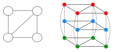
Unlike Max-Cut, where our decision was simply binary (set A or set B), here each vertex must choose one out of k possible colors. To represent this using qubits, we employ One-Hot Encoding.
For a graph with \(n\) vertices and \(k\) colors, we need \(n \times k\) qubits in total. The qubits corresponding to a single vertex are grouped together. The critical rule is: exactly one qubit in this group can be in the \(|1\rangle\) state, while the rest must remain in \(|0\rangle\).
Example for k=3 (Red, Green, Blue):
\(|100\rangle\) 🔴
\(|010\rangle\) 🟢
\(|001\rangle\) 🔵
The \(k\)-Coloring Hamiltonian
We model the graph coloring problem using binary variables \(x_{u,c} \in \{0, 1\}\), where \(x_{u,c} = 1\) if vertex \(u\) is assigned color \(c\). The classical QUBO cost function enforces the problem’s rules through two main components:
1. Conflict Term (Edge Penalty)
This term evaluates the graph’s topology. For every edge connecting vertices \(u\) and \(v\), and for every possible color \(c\), we check if both vertices share the same color. If \(x_{u,c} = 1\) and \(x_{v,c} = 1\), the product is \(1\), which adds a penalty to the total energy. The optimizer seeks to minimize this sum, striving for a configuration with zero adjacent color conflicts.
2. Single Color Constraint (Vertex Penalty)
This term enforces our one-hot encoding logic. For every vertex \(v\), the total number of colors assigned to it (\(\sum_{c} x_{v,c}\)) must be exactly \(1\).
If a vertex receives zero colors, or multiple colors, the term inside the parentheses will be non-zero.
By squaring this deviation and multiplying it by a massive penalty constant (\(A\)), we construct an energy barrier that heavily discourages the optimizer from violating the “one color per vertex” rule.
def graph_coloring_h(
    edges: list[tuple[int, int]],
    num_nodes: int,
    num_colors: int,
    penalty: int,
    qubits: Quant,
) -> Hamiltonian:

    qubits = [qubits[i * num_colors : (i + 1) * num_colors] for i in range(num_nodes)]

    conflict = sum(
        sum(B(qubits[u][c]) * B(qubits[v][c]) for c in range(num_colors))
        for u, v in edges
    )

    one_hot_restriction = sum(
        (sum(B(qubits[v][c]) for c in range(num_colors)) - 1) ** 2
        for v in range(num_nodes)
    )

    return conflict + penalty * one_hot_restriction
Graph Coloring Instance
Let’s define our test graph (4 nodes, 5 edges) and display it with a valid 3-coloring:
edges = [(0, 1), (0, 2), (1, 2), (1, 3), (2, 3)]
num_nodes = 4
num_colors = 3

# Show an example valid coloring
plot_k_coloring_graph(
    edges,
    num_nodes,
    num_colors,
    [0, 0, 1, 0, 1, 0, 0, 0, 1, 1, 0, 0],
    title="Example Valid 3-Coloring",
)
First Attempt: Standard Mixer
We first try QAOA with the standard Pauli-X mixer and Hadamard initial state. This explores the full \(2^{nk}\) Hilbert space rather than just the valid one-hot subspace. The penalty term enforces the one-hot constraint.
penalty = 2
k_coloring = partial(graph_coloring_h, edges, num_nodes, num_colors, penalty)

res, result = qaoa(
    problem_h=k_coloring,
    mixer_h=default_mixer_h,
    initial_state=H,
    num_qubits=num_nodes * num_colors,
    p=6,
)

print(res)
display(result.histogram("bin", hamiltonian=k_coloring))

plot_k_coloring_graph(
    edges,
    num_nodes,
    num_colors,
    result.most_frequent_state(),
)
 message: Return from COBYLA because the trust region radius reaches its lower bound.
 success: True
  status: 0
     fun: 5.544658237597814
       x: [ 1.559e+00 -9.054e-02  3.891e-01  1.440e+00  4.284e-01
            5.227e-01  4.239e-01  5.970e-01  3.112e-02  1.996e-01
            1.114e-01  1.572e-01]
    nfev: 234
   maxcv: 0.0
XY Mixer in the One-Hot Subspace
Using the standard mixer Hamiltonian (\(\sum X_i\)) for this problem introduces a significant challenge. The Pauli-X operator flips qubits individually.
Applying \(e^{-i\beta X}\) to a valid state like \(|100\rangle\) generates superpositions involving invalid states, such as \(|110\rangle\) (a vertex with two colors) or \(|000\rangle\) (a vertex with no colors). This inadvertently expands our search space from \(k^n\) (valid configurations) to \(2^{nk}\) (the entire Hilbert space). This drastically reduces optimization efficiency and necessitates a huge number of layers (\(p\)) to guide the system back to valid states.
To restrict the algorithm to only explore valid configurations, we use the XY Mixer (often called the Ring Mixer).
The XY Mixer evolution operator acts on pairs of qubits, swapping the states \(|01\rangle \leftrightarrow |10\rangle\) while leaving \(|00\rangle\) and \(|11\rangle\) unchanged:
Implementation in QAOA:
We connect the \(k\) qubits of a single vertex in a ring topology (qubit 1 connects to 2, 2 connects to 3, … and the last connects back to 1). Applying the XY Mixer across this ring ensures the single \(|1\rangle\) state (the vertex’s current color) can only “jump” to an adjacent color slot. This creates a superposition of valid color assignments without ever introducing a second color or eliminating the existing one.
def xy_mixer_h(qubits: Quant) -> Hamiltonian:
    """XY-Mixer Hamiltonian"""

    n = len(qubits)
    ring = [(i, (i + 1) % n) for i in range(n)]

    with obs():
        return sum(X(i) * X(j) + Y(i) * Y(j) for i, j in map(qubits.at, ring)) / 2


def graph_coloring_mixer_h(
    num_nodes: int,
    num_colors: int,
    qubits: Quant,
) -> Hamiltonian:

    qubits = [qubits[i * num_colors : (i + 1) * num_colors] for i in range(num_nodes)]

    return sum(xy_mixer_h(node) for node in qubits)
Executing the Graph Coloring Optimization
When running this subspace-restricted version of QAOA, we can no longer use a simple layer of Hadamard (\(H\)) gates for our initial_state. We must prepare an initial state that starts as a valid One-Hot configuration for every vertex.
For example, we can initialize the first color qubit of each vertex with an \(X\) gate, or use ket.qulib.prepare.w to create an equal superposition of all valid one-hot states.
def graph_coloring_initial_state(
    num_nodes: int,
    num_colors: int,
    qubits: Quant,
):
    qubits = [qubits[i * num_colors : (i + 1) * num_colors] for i in range(num_nodes)]
    for node in qubits:
        qulib.prepare.w(node)
Executing with XY Mixer
With the XY mixer and one-hot initial state, QAOA stays entirely within the valid coloring subspace. This removes the need for a penalty term (\(A=0\)) and dramatically improves convergence:
penalty = 0
k_coloring = partial(graph_coloring_h, edges, num_nodes, num_colors, penalty)

res, result = qaoa(
    problem_h=k_coloring,
    mixer_h=partial(graph_coloring_mixer_h, num_nodes, num_colors),
    initial_state=partial(graph_coloring_initial_state, num_nodes, num_colors),
    num_qubits=num_nodes * num_colors,
    p=6,
)

print(res)
display(result.histogram("bin", hamiltonian=k_coloring))

plot_k_coloring_graph(
    edges,
    num_nodes,
    num_colors,
    result.most_frequent_state(),
)
 message: Return from COBYLA because the objective function has been evaluated MAXFUN times.
 success: False
  status: 3
     fun: 0.4703870242552477
       x: [ 1.489e+00  1.730e+00  1.475e+00  3.027e-01  2.740e-01
            9.969e-01  4.157e-01  3.092e-01  2.825e-01  3.039e-01
            2.002e-01 -2.976e-01]
    nfev: 1000
   maxcv: 0.0