Quantum Optimization: Max-Cut with QAOA, VQE, and FALQON

In this tutorial, we will explore three different quantum optimization algorithms to solve the Max-Cut problem using the Ket language:

Algorithm	Approach	Description
QAOA	Hybrid Variational	Ansatz inspired by adiabatic evolution, scales well with layers (\(p\))
VQE	Hybrid Variational	Hardware-efficient ansatz with automatic gradients
FALQON	Deterministic Feedback	No classical iterative optimizer required

💡 Prerequisite: Basic knowledge of quantum computing

🔧 Environment Setup

Before we begin, let’s install the necessary dependencies. We’ll use ket-lang as our core quantum programming library.

from functools import partial
from scipy.optimize import minimize
import networkx as nx
import plotly.express as px
import plotly.graph_objects as go

import plotly.io as pio
pio.renderers.default = "notebook_connected"

# Import all elements from the Ket API
from ket import *
from ket import ket_version

ket_version()

['Ket v0.10.1',
 'libket v0.7.1 [rustc 1.97.0 (2d8144b78 2026-07-07) x86_64-unknown-linux-gnu]',
 'kbw v0.5.1 [rustc 1.97.0 (2d8144b78 2026-07-07) x86_64-unknown-linux-gnu]']

✂️ Part 1: The Max-Cut Problem

What is Max-Cut?

Max-Cut is a classic problem in graph theory. Given a graph \(G = (V, \mathcal{E})\), the goal is:

Partition the set of vertices \(V\) into two disjoint subsets \(S\) and \(\bar{S}\) such that we maximize the number of edges crossing the partition (i.e., edges with one endpoint in \(S\) and the other in \(\bar{S}\)).

Formally, we want to maximize:

\[ \text{cut}(S, \bar{S}) = |\{(u, v) \in \mathcal{E} : u \in S, v \in \bar{S}\}| \]

Why is it hard?

The number of possible partitions grows exponentially with the number of vertices: for \(n\) vertices, there are \(2^{n-1}\) distinct partitions. Checking all of them is impractical even for moderately sized graphs.

Why is it interesting for quantum computing?

Max-Cut is a paradigmatic problem for quantum optimization algorithms because:

• It maps directly to a quantum Hamiltonian (Pauli operators)

• It serves as a benchmark for NISQ (Noisy Intermediate-Scale Quantum) devices

• It has real-world applications in VLSI circuit cutting, statistical physics, and machine learning

Intuitive Example

Imagine a social network where edges represent conflicts between people. We want to divide the group into two teams such that the maximum number of conflicts are placed between the teams (rather than inside them).

Available Instances

For this tutorial, we’ve prepared six graphs of increasing complexity. You can swap the instance at any time to see how the algorithms behave!

# ================================================================
# GRAPH INSTANCES
# ================================================================

graphs = {
    # number of nodes: edges
    # Instance 1: Simple Ring (4 nodes)
    #              Trivial solution: alternating colors. Optimal = 4 cut edges.
    4: [(0, 1), (1, 2), (2, 3), (3, 0)],
    # Instance 2: Butterfly (5 nodes), geometric frustration
    #              The triangle (0,1,2) prevents a perfect coloring (odd cycle).
    5: [(0, 1), (0, 2), (1, 2), (2, 3), (2, 4), (3, 4)],
    # Instance 3: Triangular Prism (6 nodes), 3-regular graph
    #              Two triangles connected by lateral edges.
    6: [(0, 1), (1, 2), (2, 0), (3, 4), (4, 5), (5, 3), (0, 3), (1, 4), (2, 5)],
    # Instance 4: Cube (8 nodes), hypercube topology
    #              3-regular graph with 12 edges. Optimal = 8 cut edges (bipartite!).
    8: [(0, 1), (1, 2), (2, 3), (3, 0), (4, 5), (5, 6), (6, 7), (7, 4), (0, 4), (1, 5), (2, 6), (3, 7)],
    # Instance 5: Petersen Graph (10 nodes), classic benchmark
    #              Famous for being 3-regular, highly symmetric and internally connected.
    10: [(0, 1), (1, 2), (2, 3), (3, 4), (4, 0), (0, 5), (1, 6), (2, 7), (3, 8), (4, 9), (5, 7), (7, 9), (9, 6), (6, 8), (8, 5)],
    # Instance 6: 3x4 Grid (12 nodes), lattice topology
    #              Simulates square grid interactions, common in superconducting quantum hardware.
    12: [(0, 1), (1, 2), (2, 3), (4, 5), (5, 6), (6, 7), (8, 9), (9, 10), (10, 11), (0, 4), (4, 8), (1, 5), (5, 9), (2, 6), (6, 10), (3, 7), (7, 11)],
}

Graph and Cut Visualization

The plot_maxcut function below serves two purposes:

1. No result (result=None): shows the original graph with all nodes in the same color.

2. With result (result=<integer>): interprets the integer as an \(n\)-bit binary string, colors the nodes in set \(S\) 🔵 blue and those in set \(\bar{S}\) 🔴 red, and highlights the cut edges with dashed red lines.

Binary representation: An \(n\)-qubit state measured as integer r maps qubit \(i\) to bit \(i\) of the binary representation of r. Bit 0 → vertex in blue group; bit 1 → red group.

def plot_maxcut(n: int, result: int | None = None):
    """
    Plots the graph with n vertices, highlighting the cut if 'result' is provided.

    Parameters
    ----------
    n      : number of vertices (selects the graph from the `graphs` dictionary)
    result : n-bit integer representing the partition (optional)
               - bit 0 → blue group (set S)
               - bit 1 → red group (set S̄)
    """
    G = nx.Graph()
    G.add_edges_from(graphs[n])
    pos = nx.spring_layout(G, seed=42)

    # ── Node colors ────────────────────────────────────────────────────────
    node_colors = ["#00dfff"] * n  # default blue (no result)
    bin_str = None
    if result is not None:
        bin_str = bin(result)[2:].zfill(n)
        node_colors = ["#EF553B" if bit == "1" else "#00dfff" for bit in bin_str]

    # ── Edge classification ─────────────────────────────────────────────────
    uncut_x, uncut_y = [], []
    cut_x, cut_y = [], []
    for u, v in G.edges():
        x0, y0 = pos[u]
        x1, y1 = pos[v]
        # An edge is "cut" if the two nodes have different bits
        if bin_str is not None and bin_str[u] != bin_str[v]:
            cut_x.extend([x0, x1, None])
            cut_y.extend([y0, y1, None])
        else:
            uncut_x.extend([x0, x1, None])
            uncut_y.extend([y0, y1, None])

    # ── Plotly traces construction ──────────────────────────────────────────
    traces = []
    if uncut_x:  # uncut edges: solid gray
        traces.append(
            go.Scatter(
                x=uncut_x,
                y=uncut_y,
                line=dict(width=3, color="#888"),
                hoverinfo="none",
                mode="lines",
            )
        )
    if cut_x:  # cut edges: dashed red
        traces.append(
            go.Scatter(
                x=cut_x,
                y=cut_y,
                line=dict(width=3, color="#EF553B", dash="dot"),
                hoverinfo="none",
                mode="lines",
                name="Cut edge",
            )
        )

    # ── Node trace ─────────────────────────────────────────────────────────
    traces.append(
        go.Scatter(
            x=[pos[v][0] for v in G.nodes()],
            y=[pos[v][1] for v in G.nodes()],
            mode="markers+text",
            text=list(G.nodes()),
            textposition="middle center",
            textfont=dict(color="white", size=16),
            marker=dict(size=45, color=node_colors, line_width=2),
        )
    )

    # ── Cut count (if result exists) ────────────────────────────────────────
    cut_count = ""
    if bin_str is not None:
        n_cut = sum(1 for (u, v) in G.edges() if bin_str[u] != bin_str[v])
        cut_count = f", {n_cut} edges cut out of {len(graphs[n])}"

    title = (
        ("Max-Cut Result" + cut_count)
        if result is not None
        else f"Graph with {n} vertices"
    )

    fig = go.Figure(
        data=traces,
        layout=go.Layout(
            title=title,
            title_x=0.5,
            showlegend=False,
            xaxis=dict(showgrid=False, zeroline=False, showticklabels=False),
            yaxis=dict(showgrid=False, zeroline=False, showticklabels=False),
            width=500,
            height=500,
        ),
    )
    fig.show()

# Initial graph visualization (no result)
plot_maxcut(4)

🧮 Part 2: Quantum Mapping — Hamiltonians

The first step to solving Max-Cut quantumly is to translate the problem into the language of quantum mechanics. Instead of maximizing the number of cut edges, we want to minimize the energy of a physical system described by an operator called the Hamiltonian.

Variable Encoding

Each vertex \(v_i\) is mapped to a qubit \(i\). The state of each qubit (0 or 1) indicates which group the vertex belongs to. Measuring the system at the end of the circuit reveals the partition found.

🟢 Cost Hamiltonian (\(H_C\))

The Cost Hamiltonian encodes the Max-Cut objective function using the Pauli-Z operator (which has eigenvalues \(+1\) and \(-1\) corresponding to qubits in state \(|0\rangle\) and \(|1\rangle\)).

For each edge \((a, b) \in \mathcal{E}\), the product \(Z_a Z_b\) equals:

• \(+1\) if the vertices are in the same group (edge not cut)

• \(-1\) if the vertices are in different groups (edge cut)

Therefore, the Hamiltonian:

\[H_C = -\frac{1}{2}\sum_{(a,b) \in \mathcal{E}} \left(1 - Z_a Z_b\right)\]

evaluates to \(-1\) for each cut edge and \(0\) for each uncut edge. Minimizing \(H_C\) is equivalent to maximizing the number of cut edges!

plot_maxcut(4, 0b1011)

🟡 Mixer Hamiltonian (\(H_M\))

To allow the algorithm to explore the state space and avoid getting stuck in a local minimum, we need a second Hamiltonian that does not commute with \(H_C\). The standard choice is the sum of Pauli-X operators (quantum NOT gate) on all qubits:

\[H_M = \sum_{q} X_q\]

The non-commutativity \([H_C, H_M] \neq 0\) ensures that the alternating evolution of the two Hamiltonians creates quantum interference, efficiently exploring the solution space.

Implementation in Ket

In Ket, Hamiltonians are constructed inside a {func}\~ket.gates.obs`block, which creates a{class}`~ket.expv.Hamiltonian`` object — an algebraic representation of the operator that can be used both to calculate expected values and to generate time-evolution unitaries \(e^{-i t H}\).

def cost_h(edges: list[tuple[int, int]], q: Quant) -> Hamiltonian:
    """
    Builds the Max-Cut Cost Hamiltonian:
        H_C = -1/2 * Σ_{(a,b) ∈ E} (1 - Z_a·Z_b)

    The `with obs()` block tells Ket we are building an observable
    (not executing gates in the circuit). The result is a Hamiltonian
    object that can be used in `evolve()` or `exp_value()`.

    Parameters
    ----------
    edges : list of graph edges, e.g. [(0,1), (1,2), ...]
    q     : qubit register allocated in the current process
    """
    with obs():
        # For each edge (a,b), (1 - Z_a*Z_b) equals 2 if the edge is cut, 0 otherwise.
        # Summing and dividing by -2 gives -1 per cut edge (minimization ↔ maximization).
        Hc = sum(1 - Z(q[a]) * Z(q[b]) for a, b in edges)
    return -Hc / 2

def mixer_h(nodes: Quant) -> Hamiltonian:
    """
    Builds the Mixer Hamiltonian:
        H_M = Σ_q X_q

    The X operator (Pauli-X = NOT gate) creates transitions between states |0⟩ and |1⟩,
    allowing the system to explore different vertex colorings.
    Its non-commutativity with Z is fundamental: [X, Z] = 2iY ≠ 0.

    Parameters
    ----------
    nodes : list/Quant of qubits to be connected by the mixer
    """
    with obs():
        Hm = sum(X(q) for q in nodes)
    return Hm

1️⃣ QAOA — Quantum Approximate Optimization Algorithm

How QAOA Works

QAOA was proposed by Farhi, Goldstone, and Gutmann in 2014 as a hybrid quantum-classical method for combinatorial optimization problems.

The algorithm prepares an initial state and applies \(p\) layers of alternating unitary evolutions:

1. Cost Evolution: \(e^{-i \gamma H_C}\) (adds phases according to the cost function)

2. Mixer Evolution: \(e^{-i \beta H_M}\) (creates transitions between states)

The parameters \(\gamma\) and \(\beta\) are optimized by a classical algorithm (like COBYLA) to minimize the expected value \(\langle H_C \rangle\).

def qaoa_ansatz(edges, qubits, gamma, beta):
    """
    Builds the QAOA variational circuit with p layers.

    Structure:
        1. Initial state: uniform superposition with H on all qubits
        2. For each pair (γ_k, β_k):
           a. Cost Hamiltonian evolution:  e^{-i γ_k H_C}
           b. Mixer Hamiltonian evolution: e^{-i β_k H_M}

    The `evolve(t * H)` function in Ket directly applies the matrix exponential
    e^{-i t H} to the current circuit state, without manually decomposing
    into primitive gates!

    Parameters
    ----------
    edges  : list of graph edges
    qubits : qubit register of the process
    gamma  : list of p angles γ (cost evolution)
    beta   : list of p angles β (mixer evolution)
    """
    # Step 1: prepare uniform superposition |+⟩^⊗n
    H(qubits)

    # Step 2: apply p alternating layers of cost and mixer
    for g, b in zip(gamma, beta):
        evolve(g * cost_h(edges, qubits))  # e^{-i γ H_C}
        evolve(b * mixer_h(qubits))        # e^{-i β H_M}

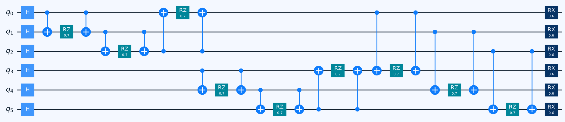
QAOA Circuit Visualization

Ket’s qulib.draw function allows us to visualize the quantum circuit that will be executed. Let’s see what a 1-layer (\(p=1\)) QAOA circuit looks like for the selected graph:

# QAOA circuit visualization for p=1 (one layer)
# Using parameters γ=0.7, β=0.3 as an illustrative example
n = 6
qulib.draw(lambda q: qaoa_ansatz(graphs[n], q, gamma=[0.7], beta=[0.3]), n, fold=-1)

Objective Function and Classical-Quantum Loop

The qaoa_objective function is called repeatedly by the COBYLA optimizer. In each call, it:

1. Creates a new Ket Process (qubit allocation in the simulator).

2. Executes the ansatz with the current parameters.

3. Calculates and returns the expected value \(\langle H_C \rangle\).

def qaoa_objective(edges, n, parameters, final=False):
    """
    Hybrid classical-quantum objective function for QAOA.

    This function is called in two contexts:
    - During optimization (final=False): returns ⟨H_C⟩ for the optimizer to minimize.
    - After convergence    (final=True): returns samples of the optimized state.

    Parameters
    ----------
    edges      : graph edges
    n          : number of vertices (= number of qubits)
    parameters : 1D vector with [γ_1,...,γ_p, β_1,...,β_p] concatenated
    final      : if True, returns samples instead of the expected value
    """
    # Split parameters into two vectors: gamma and beta
    p = len(parameters) // 2
    gamma = parameters[:p]
    beta = parameters[p:]

    process = Process(num_qubits=n, simulator="dense", execution="batch")
    qubits = process.alloc(n)

    qaoa_ansatz(edges, qubits, gamma, beta)

    if final:
        return sample(qubits)

    return exp_value(cost_h(edges, qubits)).get()

Executing QAOA

Now we run the full optimization loop. SciPy (COBYLA) will call qaoa_objective repeatedly, adjusting parameters until it converges to a local minimum of \(\langle H_C \rangle\).

# ── Configuration ─────────────────────────────────────────────────────────────
p = 2   # number of QAOA layers
dt = 0.5  # initial parameter scale

# Initialization inspired by adiabatic annealing:
#   γ increasing: small at the start, larger at the end  → cost gains importance gradually
#   β decreasing: large at the start, smaller at the end → mixer dominates early on
gamma_init = [i / p * dt for i in range(1, p + 1)]  # [dt/p, 2dt/p, ..., dt]
beta_init  = [(1 - i / p) * dt for i in range(1, p + 1)]  # [dt(1-1/p), ..., 0]

print("Initial parameters:")
print(f"  γ (cost,  increasing): {gamma_init}")
print(f"  β (mixer, decreasing): {beta_init}")

# Concatenate [γ_1,...,γ_p, β_1,...,β_p] into a single vector for SciPy
initial_params_qaoa = gamma_init + beta_init

# ── Optimization ───────────────────────────────────────────────────────────────
res_qaoa = minimize(
    partial(qaoa_objective, graphs[n], n),  # function for COBYLA to minimize
    initial_params_qaoa,
    method="COBYLA",
)

print(f"\nQAOA optimization completed in {res_qaoa.nfev} objective function evaluations.")
print(f"Final energy ⟨H_C⟩ = {res_qaoa.fun:.4f}  (lower = more cut edges)")
print(
    f"Optimal parameters: γ = {res_qaoa.x[:p].round(4)}, β = {res_qaoa.x[p:].round(4)}"
)

# ── Final result ───────────────────────────────────────────────────────────────
# Use the optimal parameters to sample the final quantum state
samples_qaoa = qaoa_objective(graphs[n], n, res_qaoa.x, final=True)

# Histogram colored by energy: darker bars = states with higher cost (better cuts)
samples_qaoa.histogram("bin", hamiltonian=partial(cost_h, graphs[n])).show()

# Visualize the cut found in the graph
best_state_qaoa = samples_qaoa.most_frequent_state()
print(
    f"\nMost probable state: {bin(best_state_qaoa)[2:].zfill(n)}  (integer: {best_state_qaoa})"
)
plot_maxcut(n, best_state_qaoa)

Initial parameters:
  γ (cost,  increasing): [0.25, 0.5]
  β (mixer, decreasing): [0.25, 0.0]

QAOA optimization completed in 99 objective function evaluations.
Final energy ⟨H_C⟩ = -6.3919  (lower = more cut edges)
Optimal parameters: γ = [0.6747 1.5856], β = [ 1.3373 -0.2674]

Most probable state: 011100  (integer: 28)

2️⃣ VQE — Variational Quantum Eigensolver

How VQE Works

VQE was originally proposed by Peruzzo et al. (2014) to calculate molecular energies, but it applies to any problem that can be mapped to a Hamiltonian.

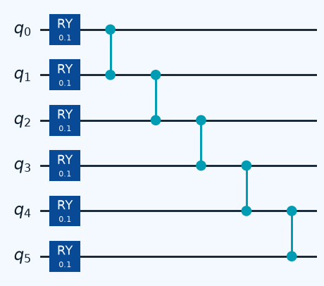
Unlike QAOA, which uses Hamiltonians that encode the problem directly into the circuit’s gates, VQE uses a Hardware-Efficient Ansatz (HEA). This ansatz consists of generic parametrized rotation gates (like \(R_Y\)) and fixed entangling gates (like \(CZ\)), which are easy to implement on real quantum hardware.

VQE relies heavily on the classical optimizer to find the right angles that minimize the energy.

def vqe_ansatz(qubits, parameters):
    """
    Hardware-Efficient Ansatz (HEA) for VQE.

    Structure of each layer:
        1. RY rotations(θ_i) on each qubit  → free parameterization
        2. CZ gates between neighboring qubits → local entanglement

    The iterator `p` steps through the parameters sequentially.
    When parameters are exhausted (next returns False), the function returns.
    This lets the number of layers be controlled simply by the length of the parameter vector.

    Parameters
    ----------
    qubits     : qubit register of the current process
    parameters : vector of angles θ (can be a list of floats or Ket Param objects)
    """
    p = iter(parameters)

    while True:
        # ── Individual rotation layer ────────────────────────────────────────
        for q in qubits:
            angle = next(p, False)
            if angle is False:  # parameters exhausted: circuit complete
                return
            RY(angle, q)  # rotation around the Y axis: Ry(θ) = e^{-iθY/2}

        # ── Entanglement layer ───────────────────────────────────────────────
        # CZ between consecutive qubits creates quantum correlations between neighboring vertices
        for i in range(len(qubits) - 1):
            CZ(qubits[i], qubits[i + 1])

def vqe_objective(edges, n, parameters, final=False):
    """
    VQE objective function with support for automatic gradients.

    Unlike QAOA, here we enable `gradient=True` in the Process so that
    Ket automatically computes ∂⟨H_C⟩/∂θ_i for each parameter.

    With gradients available, we can use SciPy's L-BFGS-B optimizer,
    which converges much faster than COBYLA on smooth cost surfaces.

    Parameters
    ----------
    edges      : graph edges
    n          : number of qubits
    parameters : vector of angles θ
    final      : if True, returns samples; if False, returns (energy, gradient)
    """
    process = Process(
        num_qubits=n,
        simulator="dense",
        execution="batch",
        gradient=not final,  # gradients only during optimization (not in the final call)
    )

    if not final:
        # Register parameters as differentiable variables of the process.
        # This allows Ket to track their derivatives automatically.
        parameters = process.param(*parameters)

    qubits = process.alloc(n)
    vqe_ansatz(qubits, parameters)

    if final:
        return sample(qubits)

    # Expected value of the energy
    result = exp_value(cost_h(edges, qubits)).get()

    # Extract gradients: ∂⟨H_C⟩/∂θ_i for each parameter.
    # Ket computes this automatically using the Parameter Shift Rule.
    grad = [p.grad for p in parameters]

    return result, grad

VQE Circuit Visualization

Let’s visualize the VQE circuit before running the optimization:

# VQE circuit visualization (one layer of n parameters)
qulib.draw(lambda q: vqe_ansatz(q, [0.1] * n), n, fold=-1)

Executing VQE

VQE uses SciPy’s L-BFGS-B optimizer, which is a second-order quasi-Newton method. It uses the gradients calculated by Ket to converge much faster than COBYLA.

Tip: The number of parameters controls the expressive power of the ansatz. With num_layers * n parameters, we have num_layers layers of RY + CZ rotations.

# ── Configuration ─────────────────────────────────────────────────────────────
num_layers = 2  # number of RY + CZ layers
num_params = num_layers * n  # total number of parameters θ

# Initialization with small random perturbations to break symmetry
import random

random.seed(42)
initial_params_vqe = [random.uniform(0.0, 0.3) for _ in range(num_params)]

print(f"VQE with {num_layers} layers × {n} qubits = {num_params} parameters")

# ── Optimization ───────────────────────────────────────────────────────────────
res_vqe = minimize(
    partial(vqe_objective, graphs[n], n),
    initial_params_vqe,
    method="L-BFGS-B",  # uses gradients provided by Ket
    jac=True,           # indicates the function returns (value, gradient)
)

print(f"\nVQE optimization completed in {res_vqe.nfev} objective function evaluations.")
print(f"Final energy ⟨H_C⟩ = {res_vqe.fun:.4f}")

# ── Final result ───────────────────────────────────────────────────────────────
samples_vqe = vqe_objective(graphs[n], n, res_vqe.x, final=True)
samples_vqe.histogram("bin", hamiltonian=partial(cost_h, graphs[n])).show()

best_state_vqe = samples_vqe.most_frequent_state()
print(
    f"\nMost probable state: {bin(best_state_vqe)[2:].zfill(n)}  (integer: {best_state_vqe})"
)
plot_maxcut(n, best_state_vqe)

VQE with 2 layers × 6 qubits = 12 parameters

VQE optimization completed in 30 objective function evaluations.
Final energy ⟨H_C⟩ = -7.0000

Most probable state: 101010  (integer: 42)

3️⃣ FALQON — Feedback-based ALgorithm for Quantum OptimizatioN

How FALQON Works

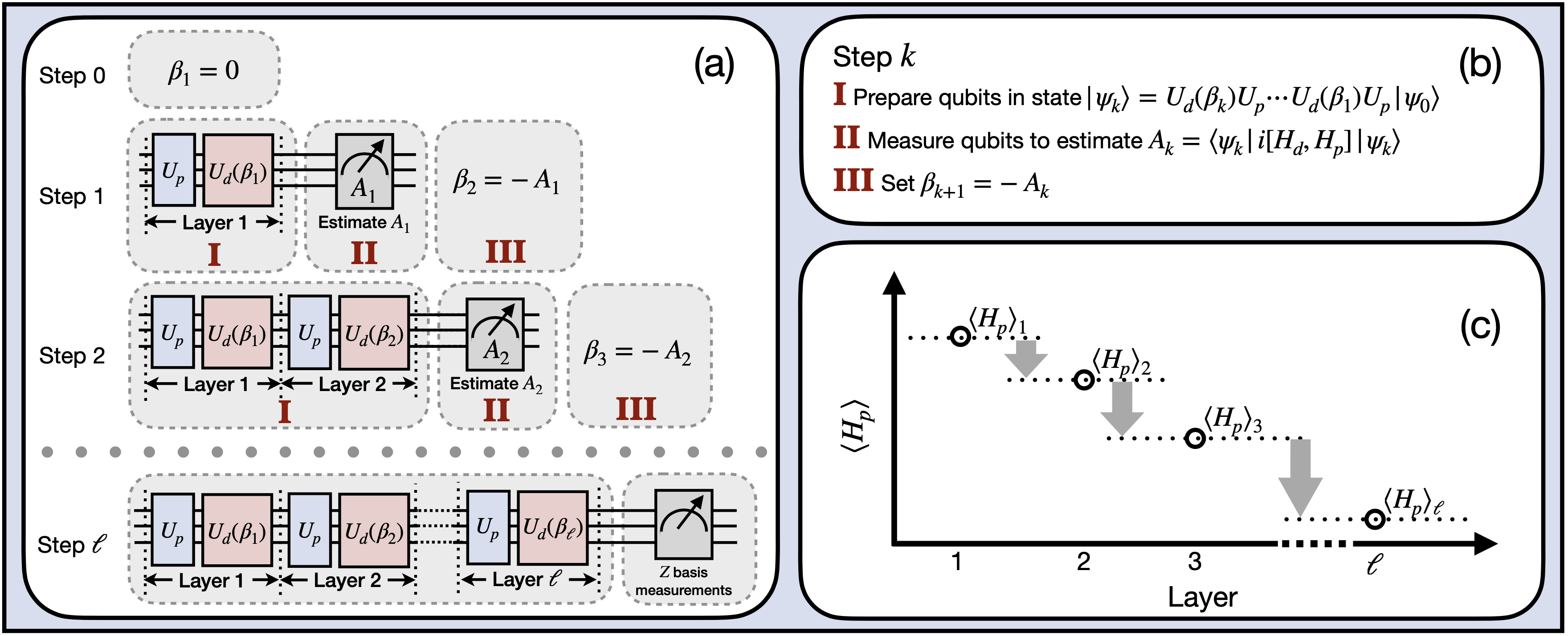
FALQON was proposed by Magann et al. (2021) as an alternative to QAOA that completely eliminates the classical iterative optimizer. Instead of adjusting parameters via minimization, FALQON uses a feedback control law based on Lyapunov theory:

If we choose the parameter \(\beta_k\) such that the energy never increases from one layer to the next, we guarantee monotonic convergence to a minimum.

The Lyapunov Feedback Law

The central theorem of FALQON establishes that if we define:

\[\beta_k = -\langle i[H_M, H_C] \rangle_k\]

where \(\langle \cdot \rangle_k\) is the expected value in the state after the \(k\)-th layer, then the energy must decrease (or remain the same) at each step:

\[\langle H_C \rangle_{k+1} \leq \langle H_C \rangle_k \quad \forall k\]

The term \(i[H_M, H_C] = i(H_M H_C - H_C H_M)\) is called the commutator Hamiltonian and measures the “flow” of energy between the two Hamiltonians.

Advantage and Limitation

✅ Advantage: Guaranteed monotonic convergence, no risk of barren plateaus or bad local minima. ⚠️ Limitation: May require more layers than QAOA to achieve the same solution quality.

execution="live" Mode in Ket

FALQON requires measuring the system between layers (to calculate \(\beta_k\)) and continuing to apply gates to the same state. This is possible in Ket using execution="live", which keeps the quantum state active in the simulator and allows interleaved reading/writing.

This is an exclusive Ket feature that greatly facilitates FALQON implementation!

def falqon_layer(edges, qubits, beta, delta_t):
    """
    Applies one FALQON layer to the current state.

    Each layer consists of:
        1. Cost evolution:  e^{-i Δt H_C}
        2. Mixer evolution: e^{-i β·Δt H_M}

    The parameter β is determined by the feedback from the previous state,
    while Δt is a fixed time step (analogous to a numerical integration step).

    Parameters
    ----------
    edges   : graph edges
    qubits  : process qubits (state preserved between calls with execution='live')
    beta    : feedback parameter computed in the previous iteration
    delta_t : time step (controls the magnitude of the evolution per layer)
    """
    evolve(delta_t * cost_h(edges, qubits))       # e^{-i Δt H_C}
    evolve(beta * delta_t * mixer_h(qubits))      # e^{-i β·Δt H_M}

def beta_h(edges, qubits):
    """
    Builds the commutator Hamiltonian for computing the feedback parameter β.

    The Lyapunov law of FALQON determines:
        β_k = -⟨i[H_M, H_C]⟩_k = -⟨i(H_M·H_C - H_C·H_M)⟩_k

    The expected value of this Hamiltonian in the current state gives exactly
    the β that guarantees the energy will not increase in the next layer.

    Note: The @ operator in Ket represents the product of Hamiltonians (composition).
    """
    Hm = mixer_h(qubits)
    Hc = cost_h(edges, qubits)
    # Commutator: [H_M, H_C] = H_M·H_C - H_C·H_M
    # Multiplied by i and negated, we get β that guarantees energy decrease
    A = 1j * (Hm @ Hc - Hc @ Hm)
    return -A

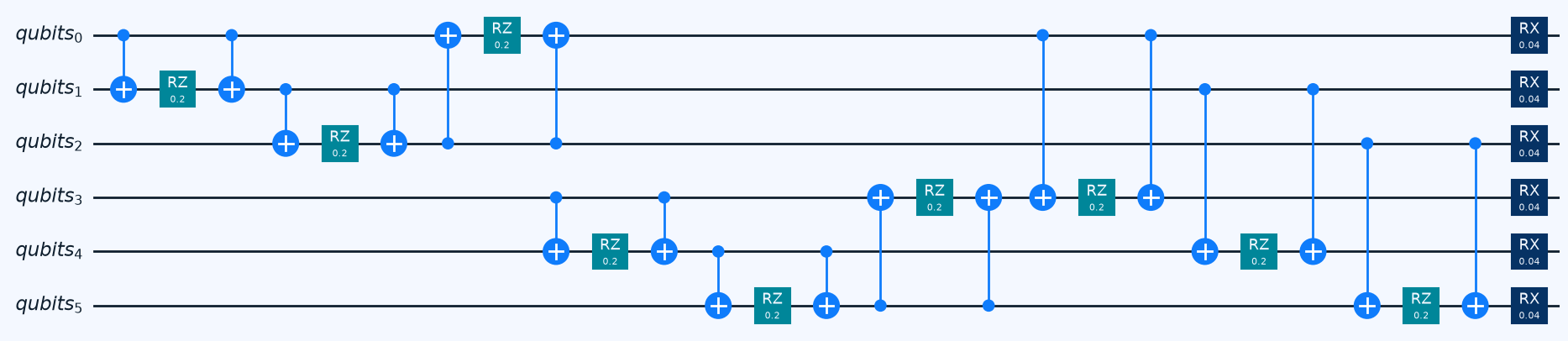
FALQON Circuit Visualization

Let’s see what a FALQON layer looks like with example parameters:

# FALQON layer visualization with β=0.1, Δt=0.2
delta_t = 0.01  # time step, small value for smooth evolution

qulib.draw(partial(falqon_layer, graphs[n], beta=0.1, delta_t=0.2), n, fold=-1)

Executing FALQON

The FALQON loop is simple and deterministic: at each iteration, we apply a layer and calculate the next \(\beta\) from the current state.

Difference from QAOA/VQE: There is no call to SciPy! The entire process is quantum-deterministic.

# ── Configuration ─────────────────────────────────────────────────────────────
num_layers = 64  # number of layers (more layers = better approximation)
delta_t = 0.01  # time step (smaller = smoother evolution, but more layers needed)

# History for convergence visualization
beta_list = [0.0]  # β₀ = 0 (no mixer evolution in the first layer)
cost_list = []     # energy ⟨H_C⟩ over the layers

# ── Process with execution='live' ──────────────────────────────────────────────
# This mode keeps the quantum state active between calls, allowing
# measurements and new gates to be interleaved on the same state.
process = Process(
    num_qubits=n,
    simulator="dense",
    execution="live",  # persistent state between operations!
)

# Initial state: uniform superposition |+⟩^⊗n
qubits = H(process.alloc(n))

print(f"FALQON: {num_layers} layers, Δt = {delta_t}")
print("Running...")

FALQON: 64 layers, Δt = 0.01
Running...

# ── Feedback loop ──────────────────────────────────────────────────────────────
for k in range(num_layers):
    # Step 1: apply the k-th layer with β computed in the previous step
    falqon_layer(graphs[n], qubits, beta_list[-1], delta_t)

    # Step 2: FEEDBACK — measure the commutator to get the next β
    # exp_value() queries the current state WITHOUT collapsing the quantum state
    beta_k = exp_value(beta_h(graphs[n], qubits)).get()
    beta_list.append(beta_k)

    # Step 3: record the current energy for monitoring
    cost_k = exp_value(cost_h(graphs[n], qubits)).get()
    cost_list.append(cost_k)

print(f"Initial energy: {cost_list[0]:.4f}")
print(f"Final energy:   {cost_list[-1]:.4f}")
print(f"Energy reduction: {cost_list[0] - cost_list[-1]:.4f}")

Initial energy: -4.5000
Final energy:   -5.7050
Energy reduction: 1.2050

# ── Final result ───────────────────────────────────────────────────────────────
samples_falqon = sample(qubits)
samples_falqon.histogram("bin", hamiltonian=partial(cost_h, graphs[n])).show()

best_state_falqon = samples_falqon.most_frequent_state()
print(
    f"\nMost probable state: {bin(best_state_falqon)[2:].zfill(n)}  (integer: {best_state_falqon})"
)
plot_maxcut(n, best_state_falqon)

Most probable state: 110001  (integer: 49)

# ── FALQON convergence charts ──────────────────────────────────────────────────
layers = list(range(1, len(cost_list) + 1))

# Energy trajectory (must be monotonically decreasing!)
fig_cost = px.line(
    x=layers,
    y=cost_list,
    labels={"x": "Layer k", "y": "⟨H_C⟩ (Energy)"},
    title="FALQON: Energy Trajectory over Layers<br><sup>Monotonic convergence guaranteed by Lyapunov's law</sup>",
    markers=True,
    color_discrete_sequence=["#636EFA"],
)
fig_cost.add_hline(
    y=min(cost_list),
    line_dash="dash",
    line_color="red",
    annotation_text=f"Minimum energy: {min(cost_list):.4f}",
)
fig_cost.show()

# Feedback parameter β evolution over layers
fig_beta = px.line(
    x=layers,
    y=beta_list[1:],  # discard initial β₀ = 0
    labels={"x": "Layer k", "y": "β_k (feedback parameter)"},
    title="FALQON: Feedback Parameter β over Layers<br><sup>Computed from the commutator i[H_M, H_C]</sup>",
    markers=True,
    color_discrete_sequence=["#EF553B"],
)
fig_beta.add_hline(y=0, line_dash="dot", line_color="gray")
fig_beta.show()

Note that the energy is monotonically decreasing, a theoretical guarantee of FALQON!

🎓 Conclusions and Next Steps

What we learned

In this tutorial, we implemented three quantum optimization algorithms using the Ket language:

Algorithm	Strength	When to use
QAOA	Physically motivated ansatz, good scaling with \(p\)	When problem structure is well known
VQE	Automatic gradients, fast convergence	When using real hardware with limited connectivity
FALQON	Guaranteed monotonic convergence, no classical optimizer	When avoiding barren plateaus is critical

Ket Features Used

• with obs(): Building Hamiltonians as quantum observables

• evolve(t * H): Exact time evolution \(e^{-i t H}\) without manual decomposition

• exp_value(H).get(): Calculating the expected value \(\langle H \rangle\)

• sample(q): Sampling the final quantum state

• process.param(*θ): Differentiable parameters for automatic gradients

• execution="batch": Efficient batch submission to the simulator

• execution="live": Persistent state between operations (essential for FALQON)